A company reports quarterly earnings well above forecasts on a Friday. Its shares rise on the news, then keep rising for weeks. Had it reported on a Tuesday, more of the move would have come on the first day. In US earnings announcements from 1984 to 2004, Friday announcements drew a 15% weaker immediate price response and a 70% stronger delayed response than those made on other weekdays, with 8% less trading volume. Fewer investors pay attention at the end of the week, and the price catches up once they return.
A behavioral finance trading strategy is a rule that buys and sells securities on a return pattern attributed to a documented investor bias, such as slow reaction to news, overconfidence or the reluctance to sell at a loss. The biases themselves, with examples from real portfolios, are covered in our guide to behavioral finance biases. Five strategies built on them have been tested repeatedly since the 1980s:
- Momentum
- Buy the stocks with the highest returns over the past 3 to 12 months and sell those with the lowest. Attributed to underreaction to news, followed by overreaction.
- Post-earnings announcement drift
- Buy after large positive earnings surprises, sell after large negative ones, and hold for up to about 60 trading days. Attributed to limited attention.
- Capital gains overhang
- Buy stocks whose holders sit on large paper gains and sell those whose holders sit on paper losses. Attributed to the disposition effect.
- Long-term reversal
- Buy the worst performers of the past three to five years and sell the best. Attributed to overreaction and extrapolation.
- Sentiment timing
- Lean against small, young, volatile and unprofitable stocks after periods of high investor optimism. Attributed to noise traders and the cost of short selling.
The returns reported in the original papers are gross of trading costs, and most shrank after publication.
Momentum and the behavioral models that explain it
Narasimhan Jegadeesh and Sheridan Titman ranked NYSE and AMEX stocks from 1965 to 1989 on their past returns. Buying the top tenth over the previous six months, selling the bottom tenth and holding for six months earned 0.95% a month before costs. Ranking on 12 months and holding for 3 earned 1.31% a month. How momentum became a standard factor next to value and quality is covered in our article on factor investing.
Systematic risk does not account for these returns, which left room for behavioral explanations. Three models published in 1998 and 1999 offered one each:
- Conservatism and representativeness. In the model of Barberis, Shleifer and Vishny, investors update too slowly after a single earnings surprise, so the price underreacts. After a run of surprises in the same direction, they conclude the company has entered a trend and overreact.
- Overconfidence and biased self-attribution. In Daniel, Hirshleifer and Subrahmanyam, investors overweight their private information. News that confirms their view raises their confidence further, news that contradicts it is put down to bad luck, and the price overshoots before it corrects.
- Slow diffusion of information. In Hong and Stein, news reaches investors gradually, so prices underreact at first. Trend-following traders then buy on the price move itself and carry it past fair value.
The Hong and Stein model predicts stronger momentum where news travels slowest. Sorting stocks by analyst coverage after controlling for size, from 1980 to 1996, the six-month strategy earned 1.13% a month among the least covered stocks and 0.72% among the most covered. The whole gap came from losers. Bad news about thinly followed companies reached prices more slowly than bad news about well-followed ones.
The behavioral models also predict that momentum reverses once prices overshoot. Jegadeesh and Titman tested both points in 2001. In the eight years after their first sample ended, 1990 to 1997, winners still beat losers by 1.01% a month, against 1.11% in 1965 to 1989. Cumulative profits reached about 11% twelve months after portfolio formation and fell back to 0.79% by month 60, so nearly all of the first year's gain was given back over the next four. The reversal was strong in 1965 to 1981 and close to zero in 1982 to 1997, and the authors described their evidence as support for the behavioral models, to be read with caution.
Momentum crashes in 1932 and 2009
Momentum loses most when a falling market turns sharply upward, because the stocks that fell hardest, which the strategy is short, rebound the most. From July to August 1932 the decile of past losers among US stocks returned 232% while past winners gained 32%. From March to May 2009 losers returned 163% and winners 8%.
The winner-minus-loser portfolio lost 60.98% in July 1932 and 74.36% in August 1932, its two worst months between 1927 and 2013. It lost 42.28% in March 2009 and 45.52% in April 2009.
What momentum costs to trade
Estimates of momentum's trading costs differ by a factor of ten. Using spread and price-impact estimates for 1980 to 1998, Lesmond, Schill and Zhou put the round-trip cost of the standard portfolio at 9.4%, against a gross return of 7.8% over six months. Korajczyk and Sadka found that price impact erased the excess return of liquidity-weighted momentum portfolios once about 5 billion dollars was invested, at December 1999 market values, and about 200 million dollars for an equal-weighted version.
AQR's own executions, close to 1 trillion dollars of trades from 1998 to 2011, showed costs less than a tenth as large as the academic estimates. On those costs, momentum broke even up to 52 billion dollars in US stocks and 89 billion dollars globally.
Post-earnings announcement drift and limited attention
Ray Ball and Philip Brown noticed in 1968 that share prices kept moving in the direction of an earnings surprise after the announcement. The trading rule built on it ranks stocks by standardized unexpected earnings (SUE), the gap between reported and expected earnings divided by the standard deviation of past surprises, then buys the top decile and sells the bottom one. From 1972 to 2005 this earned about 0.90% a month, roughly 10% a year, before costs.
Victor Bernard and Jacob Thomas traced the drift to how investors read quarterly earnings. A surprise in one quarter tends to be followed by surprises of the same sign in the next few. Prices behave as if investors expected no such persistence, so the three-day price reactions to the next four quarterly announcements can be predicted from the current quarter's earnings.
The drift is larger when investors are distracted. Friday announcements are one case. Busy days are another: when many other companies report on the same day, the immediate reaction to a firm's surprise is smaller and the later drift larger. From 1995 to 2004, the 60-day return spread between the top and bottom surprise deciles was 7.41% for announcements on high-news days and 2.81% on quiet ones.
Most of the drift sits in illiquid stocks. Value-weighted, the long-short SUE portfolio earned 0.04% a month among the most liquid stocks and 2.43% among the least liquid, and transaction costs absorbed 70% to 100% of the paper profits. It has faded since. Among stocks above the 20th percentile of NYSE market value, the drift has been absent since 2006, and among microcaps since 2016, in data running to 2019.
The disposition effect as a signal: the capital gains overhang
Investors tend to sell winners too early and hold losers too long, a pattern measured in brokerage accounts and described in our article on loss aversion. When enough holders of one stock behave this way, the price shows it. Holders sitting on gains sell into good news, so the price rises less than the news justifies. Holders sitting on losses refuse to sell on bad news, so the price falls less than it should. In both cases the price lags its fundamental value and drifts toward it later.
Mark Grinblatt and Bing Han turned this into a measurable signal. They estimated each stock's average purchase price from its trading volume and defined the capital gains overhang as the percentage gap between the current price and that reference price. In weekly regressions on NYSE and AMEX stocks from 1967 to 1996, the overhang predicted returns, and once it was included, returns over the previous 5 to 52 weeks no longer did. Outside January, the overhang implied that past winners beat past losers by about 12.5% a year. In January the sign reversed, which the authors linked to tax-loss selling.
Andrea Frazzini combined the overhang with earnings news, using reference prices drawn from mutual fund holdings from 1980 to 2002. The drift after an announcement was strongest when the news and the holders' paper gains or losses had the same sign. Buying good-news stocks with the largest paper gains and selling bad-news stocks with the largest paper losses, held for three months, produced a three-factor alpha of 2.43% a month before costs. After estimated trading costs, on stocks priced above 3 dollars, it fell to 0.89% a month.
The disposition effect does not account for all of momentum. After a stock split, the price investors paid no longer lines up with the price on the screen, and the disposition effect disappears from account-level trading data in the split stocks. Momentum in those same stocks remains. Another reference price, the 52-week high printed next to most stock quotes, has its own trading strategy, described in our article on anchoring bias.
Overreaction and long-term reversal
Long-term reversal bets against extrapolation. Werner De Bondt and Richard Thaler formed portfolios of the 35 NYSE stocks with the worst and the best returns over the previous three years, sixteen times between 1932 and 1977. Over the following 36 months the losers beat the market by 19.6% and the winners trailed it by 5.0%, a gap of 24.6%. Much of the losers' gain came in January: 8.1% in the first January after formation, 5.6% in the second and 4.0% in the third. Where the result sits among the tests of market efficiency is covered in our article on random walk theory.
Size and risk account for part of the effect. Ranking NYSE stocks on five-year returns from 1926 to 1986, extreme losers beat extreme winners by 14.0% a year in raw returns over the next five years, 9.7% after adjusting for size and 4.8% after adjusting for size and beta.
- The effect reached 7.9% a year among the smallest 40% of firms and 2.6% among the largest 20%.
- It was concentrated in January. From February to December the gap between losers and winners was not statistically significant.
Josef Lakonishok, Andrei Shleifer and Robert Vishny applied the same logic to valuation in 1994. Investors, they argued, extrapolate past earnings growth too far, so they overpay for glamour stocks and underpay for value stocks. On NYSE and AMEX stocks from 1968 to 1990, value portfolios sorted on two measures at once beat glamour portfolios by about 10 to 11% a year over five-year holding periods. The value premium's later history, including its 57.8% drawdown from 2007 to 2020, is in our article on factor investing.
Reversal also appears over a single month. Sorting US stocks on a forecast built from their past monthly returns, the extreme deciles were 2.49% a month apart from 1934 to 1987. The strategy trades so often that costs dominate it. In AQR's execution data, short-term reversal in US stocks did not break even above 9 billion dollars.
Investor sentiment and the short side of anomalies
Sentiment strategies use a market-wide reading of optimism to time when mispricing is likely to be largest. Malcolm Baker and Jeffrey Wurgler built a sentiment index from six proxies:
- the average discount on closed-end funds, which narrows when small stocks do well
- NYSE share turnover
- the number of IPOs
- the average first-day return on IPOs
- the share of equity in new securities issues
- the dividend premium, the valuation gap between companies that pay dividends and those that do not
From 1963 to 2001, after low readings of the index, small, young, volatile, unprofitable, non-dividend-paying, fast-growing and distressed stocks went on to earn high returns. After high readings they earned low returns. After low sentiment, the smallest size decile returned 2.37% a month against 0.92% for the largest, and after high sentiment the size effect disappeared. The index is updated on Wurgler's data page, with monthly values through December 2025 and five proxies, NYSE turnover having been dropped.
Most of the gain from sentiment timing comes from shorting. Across 11 well-known anomalies from 1965 to 2008, a combined long-short strategy earned 0.93% a month more after high-sentiment months, defined as months following an above-median reading of the Baker and Wurgler index. The short leg returned -0.68% a month after high sentiment and +0.65% after low sentiment, and the long leg showed no relation to sentiment. Overpricing is slower to correct than underpricing, because short selling costs money and many investors cannot do it.
Media tone moves prices for a few days. Counting negative words in the Wall Street Journal's "Abreast of the Market" column from 1984 to 1999, a one-standard-deviation rise in pessimism predicted a Dow Jones Industrial Average return 8.1 basis points lower the next day, against an average daily return of 5.4 basis points. About 6.8 basis points of that came back over the following four days.
Limits to arbitrage: why the mispricing persists
Two mechanisms limit how far professional traders correct these patterns. The first is noise trader risk: the mood of uninformed traders can push a mispriced asset further from its value before it returns, and that unpredictability deters arbitrageurs from betting heavily against them. The second is capital. Arbitrage is run by a small number of specialists investing other people's money. When a mispricing widens, their clients see losses and withdraw, which forces the arbitrageurs to sell when the opportunity is largest.
Royal Dutch and Shell show how long a mispricing can last. The two companies shared the cash flows of one group 60 to 40, so Royal Dutch's market value should have been 1.5 times Shell's. From 1980 to 1995 the ratio wandered: Royal Dutch traded about 35% below parity at its 1981 low and 10% to 12% above it by 1995, with each share's relative price following the market where it traded most.
Returns after publication and trading costs
Across 97 return predictors, portfolio returns were 58% lower after the paper describing them appeared, a result covered in our factor investing article. Costs take a further share. Across 23 well-known anomalies from 1963 to 2013, strategies that turned over less than half the portfolio each month mostly kept significant returns after costs, and only two with higher turnover did. Round-trip costs for typical value-weighted strategies exceeded 0.50%, and equal-weighted versions cost two to three times as much.
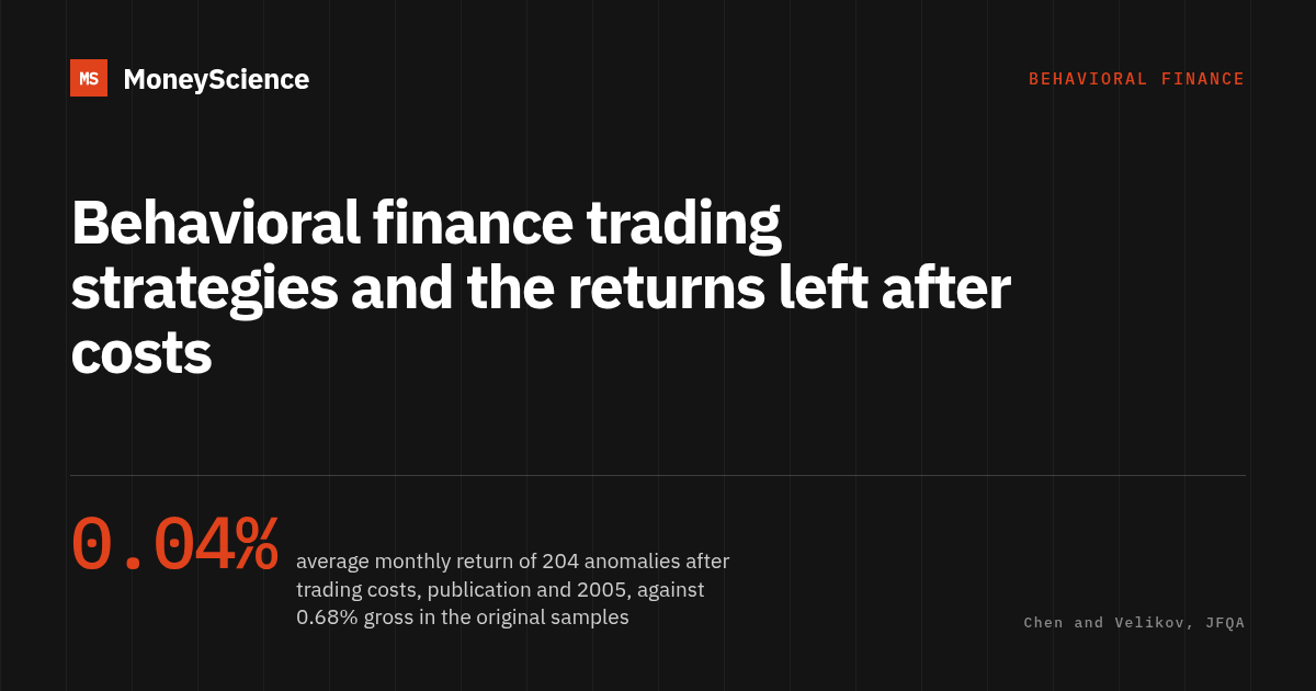
Combining both effects for 204 anomalies, the average long-short return was 0.68% a month gross in the original samples, 0.44% after designing the portfolios to cut costs, 0.09% after publication, and 0.04% after publication and 2005. The strongest anomalies kept about 0.10% a month and combinations of many signals about 0.20%, before short-selling fees estimated at 0.10% to 0.20% a month.
| Strategy | Sample | Return in the paper, before costs | Later evidence |
|---|---|---|---|
| Momentum | NYSE and AMEX, 1965 to 1989 | 0.95% a month | 1.01% a month in 1990 to 1997. Lost 74.36% in August 1932 and 45.52% in April 2009 |
| Post-earnings announcement drift | US stocks, 1972 to 2005 | 0.90% a month | Costs absorb 70% to 100%. Absent since 2006 outside microcaps |
| Capital gains overhang with earnings news | US stocks, 1980 to 2002 | 2.43% a month | 0.89% a month after estimated costs, stocks above 3 dollars |
| Long-term reversal | NYSE, 1926 to 1982 | 24.6% over 36 months | 4.8% a year after size and beta, 1926 to 1986, mostly in January |
| Sentiment timing | 11 anomalies, 1965 to 2008 | 0.93% a month more after high sentiment | The gain comes from the short leg, where borrowing fees apply |
Funds that trade on behavioral finance research
Several authors of these papers manage money on them. Lakonishok, Shleifer and Vishny founded LSV Asset Management in 1994, the year their contrarian value paper appeared. The firm runs quantitative value portfolios whose model combines value and momentum signals, and it describes its method as exploiting the judgment biases of other investors. It reported about 123 billion dollars under management for about 350 clients at June 30, 2026. Lakonishok still leads it, and Shleifer and Vishny have since retired from the firm.
Russell Fuller founded Fuller & Thaler Asset Management, now FullerThaler, in San Mateo in 1993, and Richard Thaler has been with the firm since 1998. Thaler received the 2017 Nobel Memorial Prize in Economic Sciences for his contributions to behavioral economics. The firm's stated method is to buy where investors have overreacted to bad news or underreacted to new information, and its March 2026 filing with the SEC reported 30.3 billion dollars of regulatory assets. It has been subadviser since 1998 to the Undiscovered Managers Behavioral Value Fund, a mutual fund now in the J.P. Morgan range, which held about 8.3 billion dollars in late October 2026.
This article is general information and does not recommend any fund or strategy.
Who loses money on the other side of these trades
Taiwan's stock exchange data from 1995 to 1999 tie every trade to the type of investor who made it. Individual investors' aggregate portfolio lost 3.8 percentage points a year through trading, a total equal to 2.2% of Taiwan's GDP. Of that loss, 27% came from losing trades, 32% from commissions, 34% from transaction taxes and 7% from market timing. Institutions gained 1.5 percentage points a year after costs, and foreign institutions took nearly half of those gains.
Among Taiwanese day traders from 1992 to 2006, fewer than 1% earned predictable, positive returns after fees. US evidence on overtrading, from the accounts of 66,465 households, is in our guide to behavioral finance biases, and the wider field is introduced in our overview of behavioural finance.
Stop-loss rules, a common way to take emotion out of selling, add trading of their own. Applied to a large sample of individual US stocks, tight stop-loss rules tended to underperform buying and holding because of the extra trading costs. The same 2016 MIT thesis surveyed investors on how they expected to react to large market moves. Institutional investors mostly described contrarian reactions. Individual investors, on average, described following the move.
Frequently asked questions
What is a behavioral finance trading strategy?
A trading rule that buys or sells securities on a return pattern attributed to an investor bias. The most studied are momentum, post-earnings announcement drift, the capital gains overhang left by the disposition effect, long-term reversal, and the use of investor sentiment as a timing signal. Each was first documented in historical data, and most earned less once the research was published and trading costs were counted.
Does momentum investing still work?
Momentum continued after it was published. From 1990 to 1997, past winners beat past losers by 1.01% a month in US stocks, close to the 1.11% of 1965 to 1989. It also crashes when markets rebound sharply: the winner-minus-loser portfolio lost 74.36% in August 1932 and 45.52% in April 2009. Estimates of how much money it can absorb after trading costs range from about 5 billion dollars in academic studies to 52 billion dollars in US stocks using AQR's own trade data.
Is post-earnings announcement drift still profitable?
Far less than it was. From 1972 to 2005, buying the largest positive earnings surprises and selling the largest negative ones earned about 0.90% a month before costs, and transaction costs absorbed 70% to 100% of it because the drift sat mostly in illiquid stocks. In data running to 2019, the drift has been absent since 2006 for stocks above the 20th percentile of NYSE market value, and since 2016 for microcaps.
Which behavioral biases do trading strategies exploit?
Underreaction to news, from slow updating and limited attention, is behind momentum and post-earnings announcement drift. The disposition effect, selling winners early and holding losers, creates the capital gains overhang. Extrapolation of past growth is behind long-term reversal and the value premium. Waves of optimism among less informed investors drive sentiment effects, mostly in stocks that are costly to sell short.
What are common behavioral finance errors in trading?
Three errors recur in trading records: overtrading, the disposition effect and extrapolating recent returns. In Taiwan from 1995 to 1999, individual investors' trading cost their aggregate portfolio 3.8 percentage points a year, equal to 2.2% of GDP, and fewer than 1% of day traders from 1992 to 2006 earned predictable profits after fees.