On Friday, October 16, 1987, the S&P 500 closed at 282.70. The following Monday it closed at 224.84, a fall of 20.47% in a single session. Daily S&P 500 returns from 1928 to 2025 have a standard deviation of 1.19%, which makes that Monday a move of about 17 standard deviations. A normal distribution gives a one-day loss of that size a probability of roughly 2 in 1066.
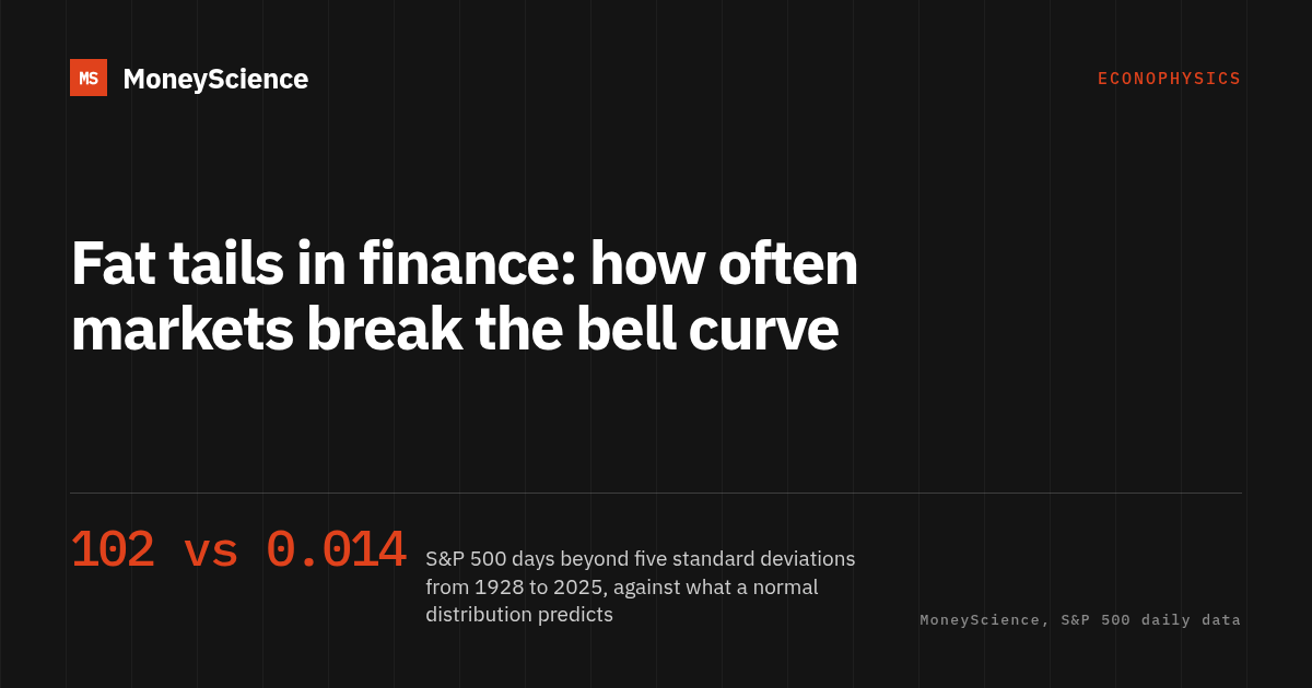
It is one of 102 days since 1928 on which the index moved by more than five standard deviations.
Fat tails are the property of a probability distribution that gives extreme outcomes much more probability than a normal distribution with the same mean and standard deviation. In finance the term describes asset returns. On the S&P 500, days beyond three standard deviations happened about six times as often as the bell curve behind many classic models allows, and days beyond five about 7,000 times as often. The effect is one of the stylized facts of asset returns found across a wide variety of markets and instruments, and measuring it is one of the main results of econophysics.
Fat tails compared with the normal distribution
A normal distribution is fixed by two numbers, the mean and the standard deviation, and its tails thin out very fast. About 68.3% of outcomes fall within one standard deviation of the mean. A move beyond three standard deviations happens once in about 370 observations. A move beyond five happens once in about 1.74 million. For daily returns, with about 252 trading days a year, that is one five-sigma day every 6,900 years.
Going from a five-sigma move to a ten-sigma move makes it about 38,000 trillion times rarer under the normal curve.
A fat-tailed distribution moves probability out of the "shoulders", the zone between one and three standard deviations, and puts it both near the center and far out in the tails. S&P 500 daily returns show both effects at once. From 1928 to 2025, 81.6% of trading days stayed within one standard deviation of the average, against 68.3% for a normal distribution. And 413 days went beyond three standard deviations, against 66 expected.
Four related terms:
- Heavy-tailed and fat-tailed
- Often used as synonyms. Some fields reserve fat-tailed for the subset of heavy-tailed distributions whose tails decay like a power law.
- Leptokurtic
- Having a kurtosis above that of the normal distribution, which in practice means a taller peak and fatter tails.
- Sigma event
- A move measured in standard deviations from the mean. A "5-sigma day" is a daily return more than five standard deviations away from the average day.
- Tail risk
- The risk of loss from outcomes in the far tail of the distribution, the ones a model built on a normal distribution treats as close to impossible.
How often the S&P 500 moved more than five standard deviations
The counts below use daily percentage changes in the S&P 500 closing level from January 3, 1928 to December 31, 2025, 24,616 trading days in all. The closes come from the long history of the index published on Yahoo Finance (^GSPC), which matches the SP500 series on FRED, sourced from S&P Dow Jones Indices, over the years FRED covers. The average daily change was 0.031% and the standard deviation 1.19%. The "normal distribution expects" column is the number of days a normal distribution with those two parameters predicts over 24,616 sessions.
| Daily move larger than | Size of move | Normal distribution expects | Days it happened | Power law with exponent 3 |
|---|---|---|---|---|
| 3 standard deviations | 3.6% | 66 | 413 | 413 |
| 4 standard deviations | 4.8% | 1.6 | 189 | 174 |
| 5 standard deviations | 6.0% | 0.014 | 102 | 89 |
| 6 standard deviations | 7.2% | 0.00005 | 62 | 52 |
| 8 standard deviations | 9.5% | 3 × 10-11 | 16 | 22 |
| 10 standard deviations | 11.9% | 4 × 10-19 | 6 | 11 |
At three standard deviations the index had about six times as many days as the normal curve expects. At five it had about 7,000 times as many: 102 days, 50 falls and 52 gains, where the normal model expects one such day in about 70 repetitions of the whole 98-year history. Further out the ratio stops meaning much, because the normal distribution's expected count becomes a number with eleven or nineteen zeros after the decimal point.
The power law column starts from the 413 three-sigma days and assumes that the number of days beyond a threshold falls with the cube of the threshold, so a threshold twice as large catches one eighth as many days. That single rule stays within about 15% of the observed count out to six standard deviations. It overshoots at eight and ten, where only 16 and 6 days are left to count and a single day more or less moves the ratio a lot.
Six days since 1928 moved more than ten standard deviations. Three were falls: October 19, 1987 (-20.47%), October 28, 1929 (-12.94%) and March 16, 2020 (-11.98%). The other three were gains in 1929, 1931 and 1933.
The 1987 crash itself inflates the standard deviation it is measured against. Measured only against the volatility of the 60 years before it, from 1928 to October 16, 1987, the crash was a 16.9 standard deviation day. Measured against the calmer 1950 to 2025 period, whose daily standard deviation was 0.99%, it was 20.6.
Kurtosis and excess kurtosis
Kurtosis is the average of the fourth power of each observation's distance from the mean, divided by the square of the variance. Because the distances are raised to the fourth power, it is dominated by the extremes. The kurtosis of a normal distribution is 3. Excess kurtosis subtracts that 3, so a normal distribution scores 0 and a positive number points to heavy tails.
Daily S&P 500 returns from 1928 to 2025 have an excess kurtosis of 17.3.
October 19, 1987 alone contributes 17.5% of the sum of fourth powers across all 24,616 days. The largest 1% of days, 246 of them, contribute 87.2%. Remove the single day of the 1987 crash and the excess kurtosis falls from 17.3 to 14.1, so one observation out of 24,616 moves the statistic by almost a fifth. With a tail exponent near 3, the fourth moment of the distribution does not exist in theory, and the sample kurtosis keeps jumping each time a new extreme day enters the history.
Kurtosis also depends on the horizon. Monthly S&P 500 returns over the same 98 years, 1,176 months, have an excess kurtosis of 7.8. Calendar-year returns, 98 of them, have an excess kurtosis of about 0. Adding up many daily returns pulls the total toward a normal shape. The fat tails therefore hit hardest where losses are counted daily, as in a leveraged fund or a bank's trading desk, and annual return tables look much calmer than daily charts.
Power laws and the inverse cubic law
A distribution has a power-law tail when the probability of a move larger than x falls in proportion to x raised to a negative power, written P(|r| > x) ≈ C x-α. The number α is the tail exponent or tail index. The lower it is, the fatter the tail. With α = 3, doubling the size of a move makes it 23 = 8 times rarer, at any size. Under the normal distribution the penalty for doubling grows as the moves get bigger: going from two to four standard deviations makes a move about 700 times rarer, going from three to six about 1.4 million times rarer.
The value of α for stock returns was pinned down in the late 1990s by physicists with access to tick data. Parameswaran Gopikrishnan, Martin Meyer, Luis Amaral and H. Eugene Stanley analyzed 40 million price changes covering every trade in all stocks on three major US markets in 1994 and 1995 and found a tail exponent of about 3. They called it the inverse cubic law. A distribution with this tail has diverging moments of order 3 and above. The S&P 500 index has the same exponent near 3 for horizons up to about four days, with a slow drift toward a normal shape at longer horizons, measured on one-minute data from 1984 to 1996, daily data from 1962 to 1996 and monthly data from 1926 to 1996. The same exponent turned up in daily data for the Nikkei and the Hang Seng.
On the 1928 to 2025 daily data, the Hill estimator, a widely used tool for measuring a tail exponent from the largest observations, returns 3.16 using the largest 1% of absolute daily moves, 2.80 using the largest 2% and 2.53 using the largest 5%. The estimate depends on where the tail is taken to begin, a known weakness of the Hill estimator, and the deepest cut, the one closest to the true tail, lands near 3.
An exponent of 3 means the variance of daily returns exists, so standard deviations and volatility are meaningful numbers. Skewness and kurtosis, which rely on the third and fourth moments, do not converge.
Mandelbrot, cotton prices and stable distributions
Economists had noticed the excess of large price changes by the 1920s. Wesley Mitchell remarked on it in 1915, and Maurice Olivier in 1926 and Frederick Mills in 1927 documented it. In 1963 Benoit Mandelbrot published The Variation of Certain Speculative Prices in the Journal of Business. He studied cotton prices: daily closes in New York from 1900 to 1905, a daily index from 1944 to 1958 and monthly prices going back to 1880. He found so many outliers that the sample second moment of price changes wandered erratically and did not settle on any value, even with long series.
His answer was to replace the normal distribution with the family of stable Paretian distributions first described by Paul Lévy. A stable distribution keeps its shape when independent copies are added together, so daily, monthly and yearly changes would all follow the same law at different scales. The normal distribution is the only member of the family with a finite variance. All the others have power-law tails with an exponent α between 0 and 2, and infinite variance. For cotton, Mandelbrot's fits pointed to α of about 1.7.
Later data broke the stable model in two places. The tail exponent of stock returns measured near 3, well outside the Lévy range of 0 to 2. And returns look more normal as the horizon lengthens, as the monthly and annual kurtosis figures above show, while a stable law with α below 2 would keep the same fat tails at every horizon. An exponent near 3 keeps the power-law tails Mandelbrot described and gives returns a finite variance.
Volatility clustering and fat tails
Large moves arrive in clusters. Counting S&P 500 days beyond four standard deviations by decade makes the pattern plain:
- 1930s: 104 days
- 1950s, 1960s and 1970s together: 4 days
- 2000s: 27 days
- 2020 to 2025: 16 days
Part of the fat tail in the full sample comes from mixing calm decades with violent ones. Robert Engle's ARCH model, which lets volatility change over time, won him a share of the 2003 Nobel prize in economic sciences for methods of analyzing time series with time-varying volatility.
Adjusting for changing volatility only partly shrinks the tails. Dividing each day's return by an exponentially weighted estimate of recent volatility (decay factor 0.94, using only data available the day before) cuts the excess kurtosis from 17.3 to 4.1. Yet 74 of the 24,366 adjusted days still fall beyond four standard deviations, where a normal distribution expects 1.5, and 26 beyond five, where it expects 0.014. October 19, 1987 remains an 11 standard deviation day even against the volatility of the weeks just before it.
Extreme value theory
Extreme value theory models only the tail of a distribution and leaves ordinary days aside. Its two main results give a limited menu of shapes for extremes, whatever the distribution underneath:
- Block maxima. Following Fisher and Tippett (1928), the largest value in a block of observations, such as the worst day of each year, converges to one of three distributions: Weibull for bounded data, Gumbel for thin tails and Fréchet for heavy, Pareto-like tails.
- Peaks over threshold. The Pickands, Balkema and de Haan theorem says that for most heavy-tailed distributions, the size of the excess above a high threshold converges to a generalized Pareto distribution. Risk managers fit that distribution to, say, every daily loss worse than 3% and read value-at-risk and expected shortfall from the fitted tail.
Extreme daily returns of an index of the most traded stocks on the New York Stock Exchange from 1885 to 1990 follow a Fréchet distribution, the case that corresponds to power-law tails.
Value-at-risk under a normal model, measured against the data
Value-at-risk (VaR) is the loss that should be exceeded on only a given share of days, such as 1%. Computing it with a normal distribution is quick, and on the 1928 to 2025 S&P 500 data it understates the loss at both the 99% and the 99.9% level:
| Measure, one day | Normal model | Actual S&P 500, 1928 to 2025 |
|---|---|---|
| 99% VaR, loss exceeded on 1% of days | -2.74% | -3.43% |
| Days worse than the normal 99% VaR | 246 expected | 456 |
| 99.9% VaR, loss exceeded on 0.1% of days | -3.66% | -7.52% |
| Days worse than the normal 99.9% VaR | 25 expected | 208 |
| Expected shortfall, average of the worst 1% of days | -3.15% | -5.07% |
At the 99% level the normal model puts the threshold 0.69 percentage points too high, about a fifth of the actual loss. At 99.9% it misses by more than half, and its threshold is breached 8.5 times as often as it should be. VaR also gives no size for the loss once the threshold is crossed. Expected shortfall measures it as the average loss beyond the threshold. The Basel Committee's 2016 market risk standard for banks moved from value-at-risk to expected shortfall under stress, a change first proposed in 2012 to better capture tail risk.
LTCM in 1998 and the 25-sigma moves of 2007
Long-Term Capital Management made its returns from judgments on interest rate spreads and market volatility, using mathematical models to find temporary price anomalies and levering its capital through repurchase agreements and derivatives. At the end of 1997 it held about 30 dollars of debt for every dollar of capital. In August 1998 Russia devalued its currency and stopped payments on its debt, interest rate spreads opened up sharply, and the fund lost 44% of its value that month. On September 23, 1998, fourteen banks and brokerage firms put 3.6 billion dollars into the fund. In testimony to Congress on October 1, 1998, Federal Reserve chairman Alan Greenspan said the models worked as long as returns followed their historical patterns, and that the losses came in a market far outside the experience built into them. With 31 dollars of assets for each dollar of capital, a loss of about 3.2% on the assets is enough to wipe out the capital.
Nine years later, in August 2007, Goldman Sachs reported that its flagship GEO hedge fund had lost 27% since the start of the year. Its chief financial officer, David Viniar, told the Financial Times the firm had been "seeing things that were 25-standard deviation moves, several days in a row". Under a normal distribution a single 25-sigma daily loss has a probability of about 3 in 10138. The largest S&P 500 day since 1928, the 1987 crash, measured 17 standard deviations.
Option prices after 1987 and the volatility smile
The Black-Scholes formula assumes that the log of the price follows a normal distribution, the random walk assumption, so a single volatility number should price every strike. S&P 500 index options have not traded that way since the crash. After October 1987, the probability distribution implied by S&P 500 option prices treated a three standard deviation decline over a year, about -36%, as roughly 10 times more likely than the lognormal model, and a four standard deviation decline, about -46%, as roughly 100 times more likely.
Expressed as implied volatility, the same prices give out-of-the-money puts a higher volatility than options struck near the current level. Plotted against the strike price, implied volatility traced a roughly symmetric smile before October 1987 and a curve tilted toward the put side after it, the pattern the options market calls the skew. Cboe publishes a SKEW index built from S&P 500 option prices, equal to 100 minus ten times the skewness those prices imply, which rises as options price more tail risk.
Tail hedging and portfolio responses to fat tails
Tail hedging means holding positions that pay off in a crash, most often out-of-the-money put options on an index, and sometimes long volatility positions. Index option prices already include the fat left tail described above, so the buyer pays for it in every period and collects only in the periods with a large fall. The result over time depends on the premium paid, the strikes chosen and whether a crash happens while the hedge is in place.
Other responses do not rely on options:
- Size leverage against the worst days on record. At five times leverage, a -20.47% day takes the whole of the capital. At the same leverage, the normal 99% one-day VaR of -2.74% shows up as a loss of 13.7% of capital.
- Stress test with real history. Replaying October 19, 1987, October 15, 2008 (-9.03%) and March 16, 2020 (-11.98%) through a portfolio shows the loss directly, without assuming a distribution.
- Expect correlations to change in a crash. Assets that move independently in quiet markets tend to fall together in a sell-off, a pattern covered in the introduction to econophysics for investors.
- Measure risk at the horizon of the portfolio. Daily returns have an excess kurtosis of 17.3 and calendar-year returns about 0. A saver who does not need to sell during a crash faces a different distribution from a leveraged trader marked to market every evening. Annual figures for a mixed portfolio, such as the drawdowns of a 60/40 portfolio, show the risk at that longer horizon.
This article is general information, not investment advice.
Questions about fat tails
What does fat tails mean in finance?
It means that large gains and losses in asset prices happen far more often than a normal distribution with the same average and standard deviation predicts. From 1928 to 2025 the S&P 500 had 102 daily moves larger than five standard deviations. A normal distribution expects 0.014 such days over the same 24,616 sessions.
How rare is a 5-sigma event in the stock market?
Under a normal distribution, a daily move beyond five standard deviations in either direction has a probability of about 1 in 1.74 million, or one day every 6,900 years at 252 trading days a year. In S&P 500 data from 1928 to 2025, with a daily standard deviation of 1.19%, there were 102 such days, 50 of them falls.
Who discovered fat tails in financial markets?
Economists including Wesley Mitchell, Maurice Olivier and Frederick Mills noted between 1915 and 1927 that price changes had too many large values for a normal curve. Benoit Mandelbrot built a model around it in 1963, in a Journal of Business paper on cotton prices going back to 1880. He proposed stable Paretian distributions with a tail exponent of about 1.7 and infinite variance. In 1998 and 1999, physicists at Boston University, including H. Eugene Stanley, measured a tail exponent of about 3 for US stocks and the S&P 500, known as the inverse cubic law, which keeps the fat tails and gives returns a finite variance.
Do fat tails mean crashes can be predicted?
Fat tails describe how often large moves happen over long periods and say little about the date of the next one. Days beyond four standard deviations came in clusters, 104 of them in the 1930s and 4 across the 1950s, 1960s and 1970s together. Risk managers use the tail to size positions, set capital and price options so that a portfolio can absorb a large move whenever it comes.